
|
|
ProbabilityReview of probability conceptsEventsIn probability, an event describes something that may or may not happen; for example, whether it will rain tomorrow, whether I will get the flu, or whether a coin will come up heads. A probability measure tells us the "size" of these events, measured in terms of how likely they are to occur. Denoting S the space of all possible events, and A, B individual events (subsets of S), the axioms of probability are
Random variablesMostly we will be thinking about probability in terms of variables. A random variable This view allows us to specify probabilities involving Continuous-valued random variables are a bit more subtle, and involve probability density functions rather than mass functions. In essence, a probability density function is the amount of probability "per unit area" ( Common DistributionsBernoulli and Multinomial DistributionsThe most common types of discrete random variable distributions are Bernoulli and multinomial distributions. The Bernoulli distribution is defined for binary-valued random variables, i.e., Gaussian DistributionsThe Gaussian distribution is perhaps the most common distribution for continuous-valued random variables. The Gaussian probability density function is given by
The multivariate Gaussian is a Gaussian distribution defined for a Just as the square root of the variance was helpful in representing the spread in one dimension, the matrix square root can help us understand the shape and size of the uncertainty in This helps us see two special cases of the Gaussian distribution. A fully general covariance matrix has ellipsoidal uncertainty shapes; a diagonal covariance looks like an axis-aligned ellipse (no rotation), and a spherical Gaussian has a "scalar" covariance (a scalar times an identity matrix, or diagonal with all the same value). We can draw samples from a multivariate Gaussian easily using this construction, by first sampling from a unit-variance
Density estimationSince machine learning is primarily concerned with adapting to observed data, most of our probability models are likely to be estimated from data. HistogramsA histogram is a simple method of estimating and visualizing a probability density function. We bin the observed data and report the fraction of data falling into each bin. This can be interpreted as a piecewise-constant estimator of the probability density function. Maximum likelihood methodsOverfitting in density estimation
Independence and Conditional IndependenceWhen two random events are independent, it greatly simplifies their probabilities. Independent events do not influence each others' outcome, e.g., if two events A,B are independent, then knowing that A occurred has no influence on the probability of B occurring: However, in practice the variables we are interested in are related to one another somehow, and so are not completely independent. A more useful type of independence relationship is conditional independence, in which two or more variables influence one another only through some intermediary variable. For example, our two events A,B may be independent of one another once we control for some cause C: |

 may take on values
  , each of which constitutes an "event", for example
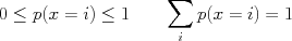
  . The values of random variables are exhaustive and mutually exclusive, meaning that
  or
or  to indicate generic values for random variable
  , etc. By the axioms of probability, and since the outcomes of x are disjoint events, we have that
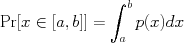
 ). An event is defined as the variable
  , and its probability mass is defined as the integral of the density over that set:
 A probability density function can be greater than 1, as long as it is only over a small area; the axioms of probability dictate that the probability mass, or integral of the density, must be less than 1.
 , and parameterized by a single parameter
  . Multinomial random variables generalize Bernoulli RVs, taking on one of
  values and parameterized by a vector of probabilities representing the probability of each outcome.
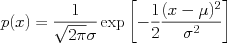 Univariate (one-dimensional) Gaussian distributions are parameterized by two scalar numbers, a mean
  and variance
  (sometimes characterized by its square root
  , the standard deviation). The mean indicates the center of the Gaussian's characteristic bell-curve shape, and equals the average or expected value of the variable
  , or equivalently a collection of
 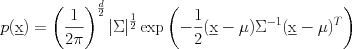 characterized by a mean vector
  covariance matrix
  representing the shape and spread of the data. The dependence on
  (in the exponential) is a quadratic form, and the shape of the equally-probable contour lines are ellipses.
 using its eigenvector decomposition, so that
  is a diagonal matrix of eigenvalues and
  is a unitary matrix. Then, the generalization of the standard deviation is
  , where
  represents a scaling and
  a rotation.
 . In general, this means that the joint probabilities factor into a product:
 . (This is an assumption about the structure of the joint distribution.)