Regression problems
Regression is a type of supervised learning task in which the target variable is real-valued.
For example, we may wish to predict the sale price of a house,  , given some of its observable characteristics, e.g.,
 : house size, in square footage
 : location, distance from the coast

We are likely to base our prediction of the sale price , and its relationship to the observable features  , on some set of training data, for example historical sales data. For simplicity of our plots, we will initially assume a single feature (e.g., size), allowing us to plot our historical data as points
  in a scatter plot, and to plot a predictor, or function
  from the observed features to the predicted value of .
| Mini: PHP-GD image library not found. Exiting. | Mini: PHP-GD image library not found. Exiting. | Mini: PHP-GD image library not found. Exiting. |
| Scatter plot of training data | Linear function f(x) | Nonlinear function f(x) |
We will initially focus on linear regression, in which our prediction about y is in the form of a linear function of the observed features , for example:
 It is helpful to define all of our variables in a matrix form; this will allow us to write very compact equations, and will also translate well into Matlab syntax. For example, defining the "zeroth feature"
  , we can write
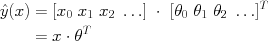 where
where  ,
,  are vectors formed by concatenating the features (respectively parameters) together.
The data that we will use for training consist of a number of examples (for example, houses that have been recently sold, or recent stock behavior); we will index each example by a parenthesized super-script:  . (The parentheses differentiate the indexing from, for example, taking a number to a power, such as
  for the square of x.
We again can vectorize an entire collection of data to be used for training into a matrix shorthand:
for the square of x.
We again can vectorize an entire collection of data to be used for training into a matrix shorthand:
 We have chosen to represent each row of X as a training example (the values of each feature observed for a particular datum, such as a single house in the historical set), while each column indicates a particular feature. The first column (of all ones) indicates "feature zero", a constant value that we prepend to our features to manage the offset term; each subsequent column represents the values of a particular feature (size, distance, etc.) that are observed across examples in the training data.
Note that the most potentially confusing difference in syntax for most presentations is a result of transposition of one or more of these quantities. It is helpful to keep in mind what the correct dimensionality of each vector is: has  elements, the number of training data;
  has
has  elements, one more than there are observed features; and
  is
is  .
.
%Matlab syntax for predicting y
yhat = X * theta'; %dot product of each example datum, in a column vector
Error measures and optimization
For a given observation (x,y), we can compute the error in our prediction (also called the residual) as  :
:
| Mini: PHP-GD image library not found. Exiting. | Mini: PHP-GD image library not found. Exiting. |
Residuals, constant  | Residuals, linear |
In general, we would like to minimize the overall size of these errors. A common, and as we shall see computationally convenient choice is the Euclidean norm of the vector of residuals, or the sum of squared errors (SSE) cost:
 The cost function J(.) tells us the accuracy of a given parameter vector at predicting our training data. This is a function defined over the space of parameters ; for a two-dimensional parameter vector, we can visualize it as a surface, or use colors or contours to suggest the three-dimensional height (cost) on a 2D plot.
| Mini: PHP-GD image library not found. Exiting. | Mini: PHP-GD image library not found. Exiting. | Mini: PHP-GD image library not found. Exiting. | Mini: PHP-GD image library not found. Exiting. |
| Color Map | 3D surface | Surface + contours | Contours only |
Gradient descent
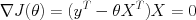
One option is to follow the local slope of  downward towards a local minimum. We can evaluate the gradient direction, i.e., the direction in which our cost function has the greatest increase; going in the opposite direction gives us the direction of greatest decrease of our cost J. This gradient will be a vector of the same dimension as :

In gradient descent, we simply initialize to some starting value of and repeatedly update by choosing a new by moving in the direction of steepest descent, e.g.,
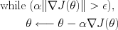 Here,
Here,  indicates that we are updating the value of using the quantity on the right. The value
  is a step-size parameter that tells us how far to move in the direction of the gradient. The choice of step size can be very important in gradient descent methods, as it often controls how fast we converge to a local minimum. Values that are too small move very slowly; values that are too large can skip over or even oscillate around local minima.
A common heuristic approach to setting the step size is to let decrease with each iteration (step), for example choosing to be inversely proportional to the iteration number.
We can see the behavior of gradient descent on the cost function J defined over parameter space (top; each point corresponds to a vector  ), and the induced predictors
  (bottom; each value of corresponds to a different linear predictor for y):
| Mini: PHP-GD image library not found. Exiting. | Mini: PHP-GD image library not found. Exiting. | Mini: PHP-GD image library not found. Exiting. | Mini: PHP-GD image library not found. Exiting. | Mini: PHP-GD image library not found. Exiting. |
| Mini: PHP-GD image library not found. Exiting. | Mini: PHP-GD image library not found. Exiting. | Mini: PHP-GD image library not found. Exiting. | Mini: PHP-GD image library not found. Exiting. | Mini: PHP-GD image library not found. Exiting. |
| Initialization | Iteration 1 | Iteration 10 | Iteration 30 | Iteration 90 |
Closed form optimum for squared error
We can solve the quadratic equation defined by the stationary point
 Rearranging gives a quadratic equation, the solution of which is the minimum squared error (MSE) estimator
 The term
  is called the (Moore-Penrose) pseudo-inverse, and compensates for the fact that X
is typically over-constrained: there is no value of theta that will exactly predict every value of y from x.
is called the (Moore-Penrose) pseudo-inverse, and compensates for the fact that X
is typically over-constrained: there is no value of theta that will exactly predict every value of y from x.
Increasing the number of features
So far we have considered linear functions of several observed features , . Suppose that we have only one feature,  , but would like our predictor to be a nonlinear function of x, for example
 We can simply define new features
  ,
,  , and so on (just as we defined
  ), and this predictor becomes simply
 In other words, it still fits the linear regression model, but in a new feature space with additional features that are deterministic functions of our observations. Applying our least-squares estimator gives polynomial fits,
  :
:
| Mini: PHP-GD image library not found. Exiting. | Mini: PHP-GD image library not found. Exiting. | Mini: PHP-GD image library not found. Exiting. | Mini: PHP-GD image library not found. Exiting. | Mini: PHP-GD image library not found. Exiting. |
| P=0 | P=1 | P=3 | P=7 | P=10 |
If we think that our target variable y is likely to be linearly related to some complex function of several observed variables, that combination can also be added as a new, observed feature.
There are two ways to view this process. First, we are creating a "more complex" functional predictor ; the set of functions we can represent is now larger (e.g., from the set of all lines to the set of all cubic polynomials). An alternative is to forget that the features are now deterministically related to one another, and to imagine that we are adding extra measurements (features) with which to predict y. In this view, we are learning a linear predictor from data, but those data lie in a higher dimensional space. (We will return to these views later, in classification.)
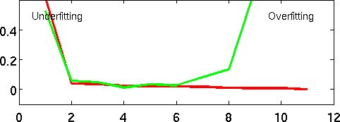
Overfitting
As we saw in our polynomial fits, for 11 data points and a degree-10 polynomial (with 11 coefficients), we can predict all of our training data exactly! And yet, something about that predictor is not satisfying -- it does not "look" like a good predictor. In fact, we have overfit to the data -- we have chosen such a complex predictor that, although it is able to reconstruct the training data, we have no faith that it will accurately predict new data.
We can see the "generalization" or test error of a predictor simply by gathering more data, and evaluating our cost function (e.g. mean squared error) on those new points (green). What we find is that, for very simple predictors (P=0,1), the performance on new test data is much like the performance on the training data. However, as the function gets more complex, the training error continues to decrease -- but the test error does not. By P=10, training error is zero, but test error is extremely high.
| Mini: PHP-GD image library not found. Exiting. | Mini: PHP-GD image library not found. Exiting. | Mini: PHP-GD image library not found. Exiting. | Mini: PHP-GD image library not found. Exiting. | Mini: PHP-GD image library not found. Exiting. |
| P=0 | P=1 | P=3 | P=7 | P=10 |
We can see this directly by plotting training and test error as a function of polynomial degree P. For very simple predictors, we are unable to capture the complexity of the dependence between x and y; but for overly complex predictors, we memorize the values of y at the expense of generalization.
Notionally, the "P" axis can be thought of as "complexity", and we find a similar curve whenever the complexity of our learner increases. We will see that much of the practical aspects of machine learning come down to choosing and controlling our position on this curve, increasing the complexity when under-fitting and decreasing it when overfitting.